Simulation dynamics¶

The events of a simulation are only half the story: they need to be generated and executed in the correct order. This is the job of the dynamics classes, the sub-classes of Dynamics.

epydemic has two simulation dynamics, for continuous-time and discrete-time simulation. In most cases continuous time (stochastic) dynamics is the correct choice, but we explain below in detail how they differ.

Continuous-time (stochastic or Gillespie) dynamics¶

A StochasticDynamics is a continuous time simulator. It maintains a joint probability distribution defining the probability of a given event occurring in a given time interval into the future. It draws from this distribution, advances the simulation time by the chosen interval, runs any posted events that should have occurred before this time, and then chooses an element on which to run the event. This technique is known as Gillespie simulation.

Let’s define a variant of SIR extended to capture the contents of all its loci:

class MonitoredSIR(SIR):
    '''An SIR model that tracks all its compartments.'''

    def build(self, params):
        super().build(params)
        self.trackNodesInCompartment(SIR.SUSCEPTIBLE)
        self.trackNodesInCompartment(SIR.REMOVED)

We can set up a single simulation of this model under stochastic dynamics very easily:

# network topological parameters (for an ER network)
N = int(1e5)
kmean = 50

# set up the simulation
param = dict()
param[ERNetwork.N] = N
param[ERNetwork.KMEAN] = kmean
param[SIR.P_INFECTED] = 0.001
param[SIR.P_INFECT] = 0.0001
param[SIR.P_REMOVE] = 0.001
param[Monitor.DELTA] = 1

e = StochasticDynamics(ProcessSequence([MonitoredaSIR(), Monitor()]),
                       ERNetwork())
rc = e.set(param).run()

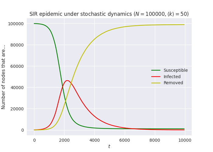
At each event the dynamics will choose what event should happen next, and after how much time, based on the rates at which events can occur. A rate is simply the probability of an event of a given type happening (taken from the experimental parameters) multiplied by the number of possible sites for the event to happen (taken from the size of the locus at which the event occurs). Plotting the results we get:

This approach to simulation is both efficient and statistically exact, which make it generally the default choice for simulations inn epydemic. Occasionally, though, we want to run experiments differently.

Discrete-time (synchronous) dynamics¶

A SynchronousDynamics is a discrete time simulator. At each timestep it runs all the events posted before this time that remain to run, and then checks all the elements that might have an event run on them and selects those that do undergo events using the given event probability.

We can run the same model with the same parameters, and just change the simulation dynamics:

e = SynchronousDynamics(ProcessSequence([MonitoredaSIR(), Monitor()]),
                        ERNetwork())
rc = e.set(param).run()

Running this simulation will look at the important loci every unit of time and, for each element decide whether to run an infection event (for an SI edge) or a removal event (for an I node) depending on the values of the experimental parameters. Plotting the results we get:

The stochastic case is generally faster than synchronous case – often massively faster. This is unsurprising: the probability of an SI edge passing an infection (for example) is usually low in any timestep, so most of the checks that the simulation performs will fail. By contrast the stochastic dynamics “steps over” time when nothing is happening. It is also statistically exact, in that the next event (and the time until it) is chosen using all the available information relating to all previous events, rather than all the one in the previous timestep as happens in the synchronous case. This can sometimes lead to different curves even for the same parameters.

Posted events¶

Both dynamics can have “normal” (stochastic) and “posted” events. The former happen at a time determined by their distribution; the latter happen at set simulation times.

Stochastic events by their nature aren’t known to happen ahead of time. Posted events can however be posted, and then at some later point (but before the event has fired) can be determined to not be needed any more and be un-posted to remove them from the event queue.

(To un-post an event you need its event identifier, which is returned by Dynamics.postEvent(). This implies that you need to remember this information for any posted event that you might later want to un-post. This isn’t an issue in practice, as it’s usually very clear which events in a simulation might need to be un-posted, and therefore need to have their ids recorded.)

The event queue is represented as a priority queue (or priqueue) held in simulation time order. This is efficient for everything except deleting (un-posting) events, so instead when un-posting we simply set the event function to None. Accessing the queue through any of the posted event methods automatically discards any leading un-posted events, so the un-posting mechanism is transparent to client code.

Event tapping¶

For both dynamics, the processing is wrapped using the functions from the event taps interface. These include marking the start and end of the simulation, and every event fired (whether per-event, fixed-rate, or posted).